Datasets

TCGA-PRAD 美國癌症基因體圖譜計畫
GSE269244 高通量基因表達數據庫

TCGA-PRAD Volcano Plot

Description

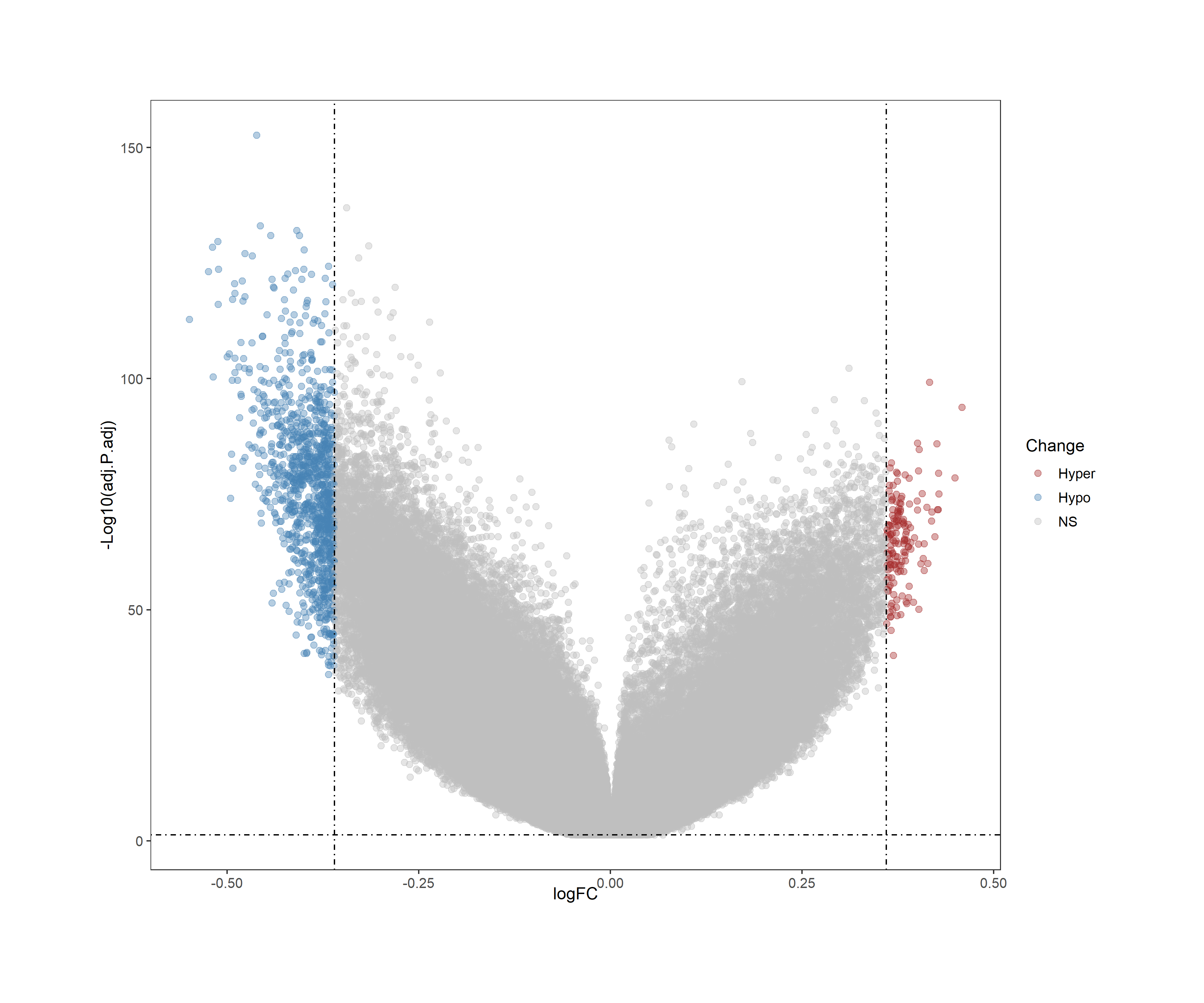
By using ChAMP package, a volcano plot can be generated to visualize the differentially methylated regions (DMRs) in the TCGA-BRCA dataset. The volcano plot displays the relationship between the significance (p-value) and the magnitude of change (fold change) of the DMRs.

Dbeta Calculation and DMR Filtering

Extensive preprocessing of GSE269244 and TCGA-PRAD methylation data was performed using the ChAMP package in R. This involved several critical steps:

Quality Control: Removal of low-quality probes, SNP-related probes, and cross-reactive probes
Normalization: BMIQ normalization to adjust for probe type bias (Infinium I vs II)
Batch Effect Correction: ComBat algorithm was applied to remove potential batch effects
Differential Methylation Analysis: Calculated differentially methylated beta values (Dbeta) between tumor and normal tissues
Statistical Filtering: Applied significance threshold of p < 0.05
Annotation: DMRs were mapped to genes based on their genomic locations and proximity to TSS (Transcription Start Sites)

The resulting differentially methylated regions (DMRs) represent critical epigenetic alterations that may drive breast cancer development and progression. Positive Dbeta values indicate hypermethylation in cancer tissues, while negative values represent hypomethylation.

Hyper/Hypo Methylation Distribution - TCGA-PRAD

Feature Distribution - TCGA-PRAD

Hyper/Hypo Methylation Distribution - GSE269244

Feature Distribution - GSE269244

Principal Component Analysis (PCA)

PCA of TCGA-PRAD

PCA of GSE269244

Joined Data Analysis

After filtering the DMRs from both datasets, we joined the two datasets to create a comprehensive dataset for further analysis. The joined dataset contains a total of 156 gene, whose similarity was calculated using GO (Gene Ontology) terms. The GO terms were obtained from the Ensembl database, and the similarity was calculated using the GOSemSim package in R.

Hierarchical clustering using simple sum

Simple Sum Clustering

Hierarchical clustering using weighted sum

Weighted Sum Clustering

Hierarchical clustering using consensus method

Consensus Clustering

Comparison of different clustering methods

Hierarchical Clustering Comparison

Machine Learning

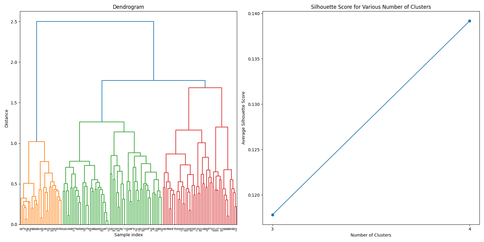
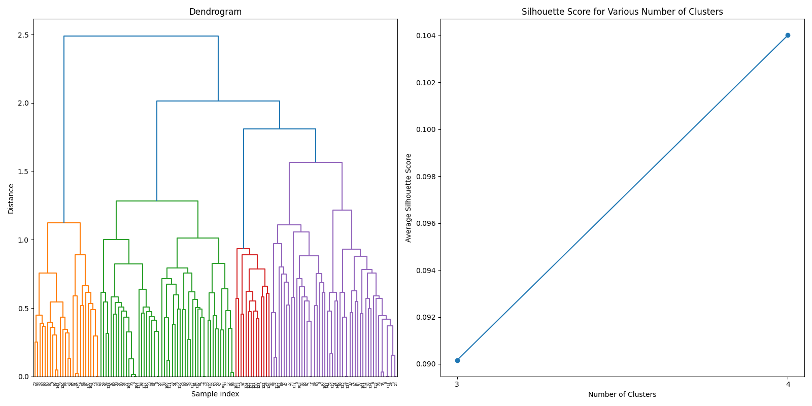
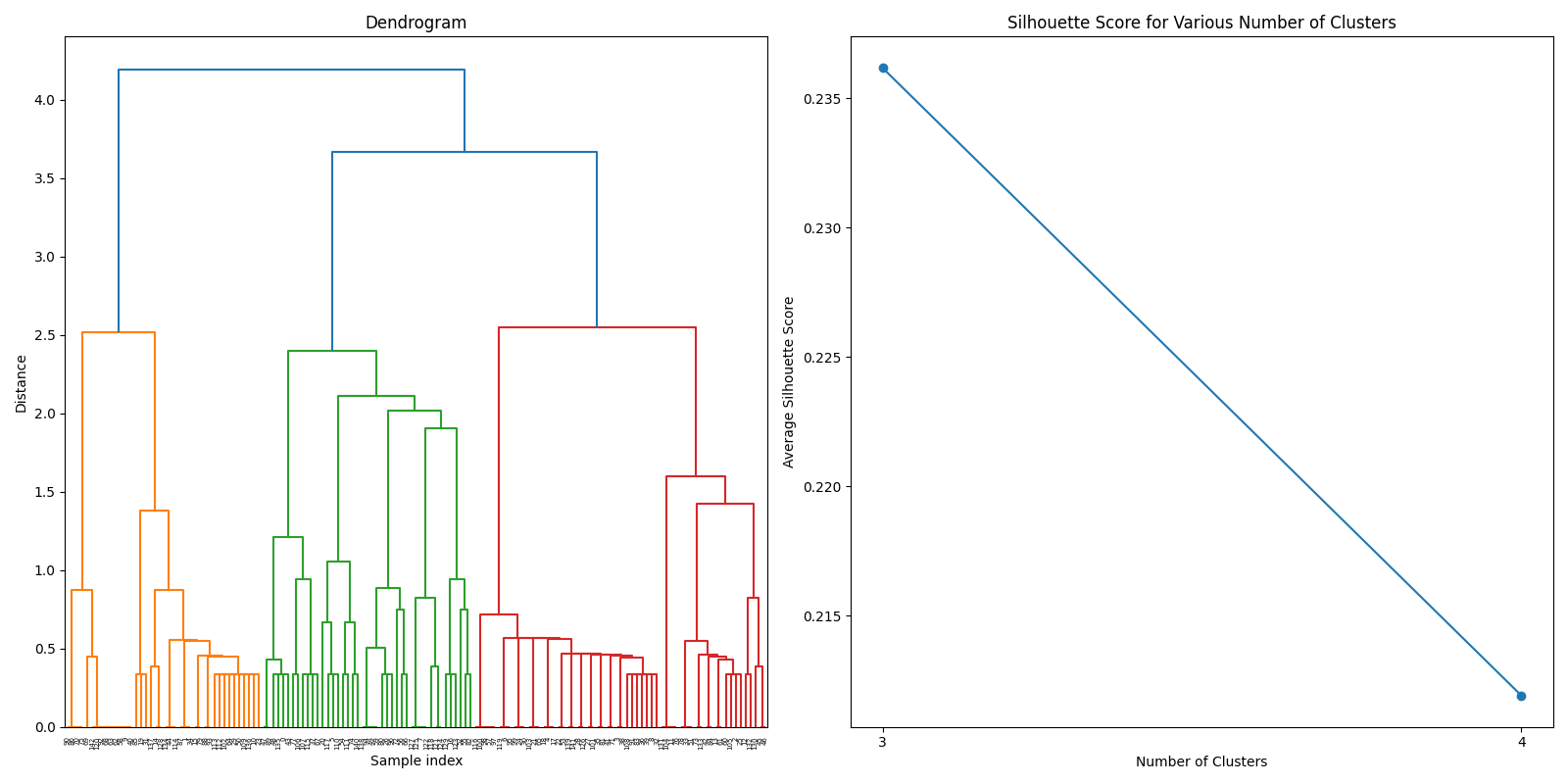
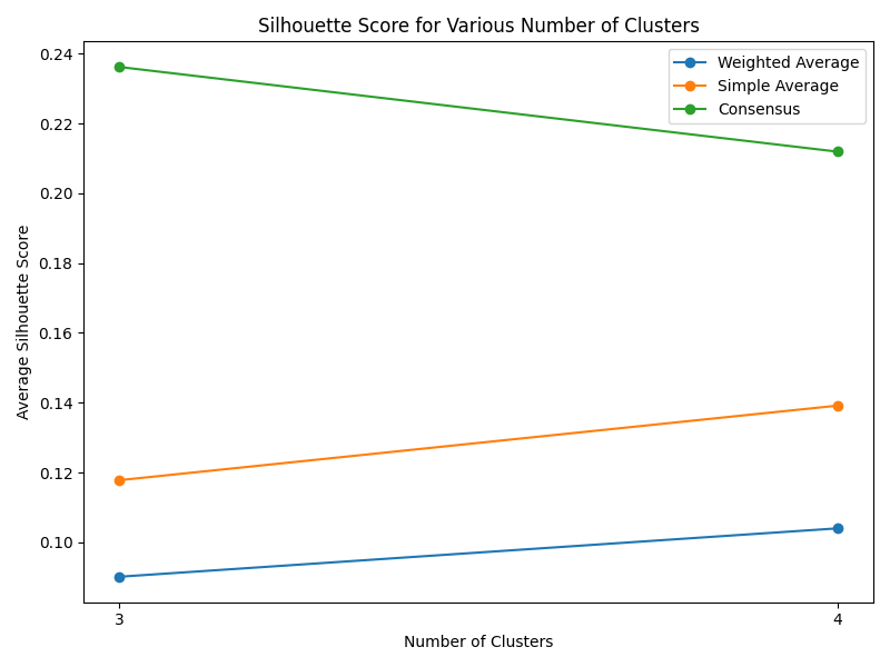
After thorough evaluation of clustering methodologies, consensus clustering emerged as the superior approach for analyzing our joined dataset due to its robustness in handling gene expression patterns. For biomarker identification, we implemented Recursive Feature Elimination (RFE) with cross-validation to systematically select the most predictive gene signatures while minimizing redundancy. This process ranked genes based on their discriminative power between cancer and normal tissue samples.

The candidate biomarkers underwent rigorous validation through an ensemble-based voting classifier architecture, which integrated predictions from multiple base learners (Random Forest, SVM, and Gradient Boosting) to improve classification stability. To enhance generalization capabilities and address potential overfitting concerns, we employed bootstrap aggregating (bagging) techniques with out-of-bag error estimation. This comprehensive machine learning pipeline delivered robust biomarker combinations with exceptional predictive performance across multiple validation datasets.

Top Gene Combinations with Highest Performance

The table below shows the gene combinations that achieved the highest classification performance:

Gene Set	Gene 1	Gene 2	Gene 3	Accuracy	Recall	Specificity	Precision	F1 Score	AUC
Set	FBXO30	KLHDC8A	PYCARD	0.898529	0.973529	0.823529	0.846478	0.905467	0.92154

RFE on Prostate Cancer Dataset